Demonstrations

There are 5 demonstrations included in the toolbox. For details on their implementation confer to the source files. Here their basics are documented.

The demonstrations are

• ghsom_demo: A simple animal data set
• ghsom_demo1: Points on a 2-dimensional grid with noise
• ghsom_demo2: Points on a 3-dimensional grid with noise
• ghsom_demo3: 4 normal distributed 2-dimensional clusters
• ghsom_demo4: music collection consisting of 77 pieces
• ghsom_demo5: musical performance data

		ghsom_demo The dataset for this demo has been published by T. Kohonen. It consists of a set of 13 animals represented by 16 attributes such as the number of legs and size. The testset is included in the toolbox and is loaded with: sD = som_read_data('animals.dat'); This is a function of the SOM Toolbox. The data format used in the GHSOM Toolbox is the same as the data structure for the SOM Toolbox. The GHSOM is trained and then labelled with: ghMap = ghsom_train(sD,'breadth',0.5,'depth',0.01); ghMap = ghsom_datalabels(ghMap, sD); The GHSOM is visualized with: ghVisu = ghsom_visualize_grid(ghMap, 'layer'); ghsom_visualize_labels(ghMap, ghVisu); And the component planes are visualized with: ghsom_visualize_grid(ghMap, 'component', [1:13]); The results are the two images: The map: 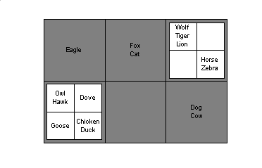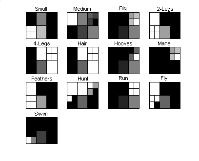The component planes: (black indicates low, white indicates high values) Back

		ghsom_demo1 The testset for this demo is a set of 100 vectors in the 2 dimensional space which are alligned on a grid with some noise. This set is used to analyze the orientation properties of the GHSOM. Notice that the orientation is maintained in sub-layers. Especially in the component plane plots this becomes very clear. The testset: 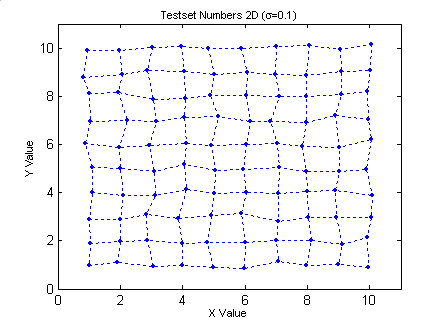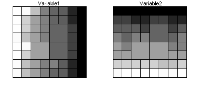The map: (x|y - labels, where x, and y are the dimensions) The component planes: Back

		ghsom_demo2 Similar as above a testset is used consisting of 100 points on a grid. The grid is three dimensional and similar to a horse saddle, to make it more difficult for the GHSOM to maintain the correct orientation on the sublayers. However from the component planes it can be seen that the orientation is maintained correctly. The testset: 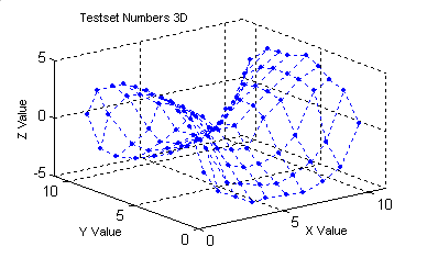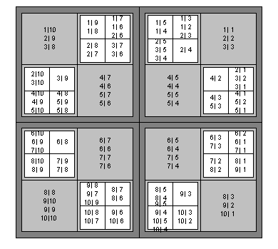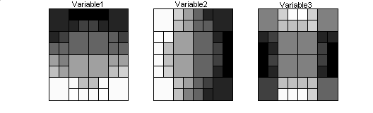The map: (x|y - labels, where x, and y are the dimensions) The component planes: Back

		ghsom_demo3 The testset for this demo consists of four normally distributed 2-dimensional clusters, with different variances. A comparision is made to the SOM. The testset: +, o, diamonds and x (starting lower right going towards upper left) 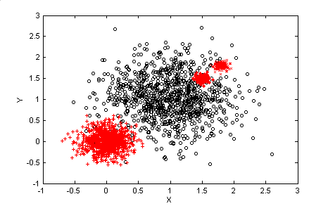An automatically (see SOM Toolbox) trained SOM: The colorcoding used coresponds to the ratio between the classes: 100% o's is plain white, 100% others is dark gray. Notice the smooth transitions between the classes. Only the most frequent member of a unit is plotted. (Note that using the "bubble" neighborhood would change this.) 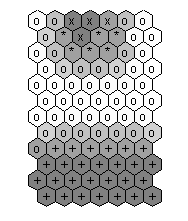The component planes and the colorcoding mentioned above (titled "Class"): Notice the very smooth and even component planes. 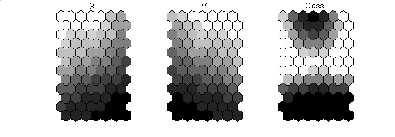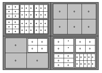The GHSOM map: The component planes and the color coded class distributions: Notice that the classes are seperated much clearer. 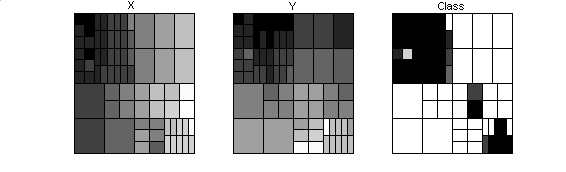Back

		ghsom_demo4 To illustrate an application of the GHSOM we use a dataset consisting of 77 pieces of music. Each piece is represented by 1200 low-level features which describe the dynamics of the loudness in frequency bands. See Islands of Music for details. The dataset is included in the toolbox and is loaded with: load music; Which loads the variable sData. The GHSOM is trained, labelled, and visualized with: ghMap = ghsom_train(sData,'breadth',0.6,'depth',0.01); ghMap = ghsom_datalabels(ghMap, sData); ghVisu = ghsom_visualize_grid(ghMap,'layer'); ghsom_visualize_labels(ghMap, ghVisu); 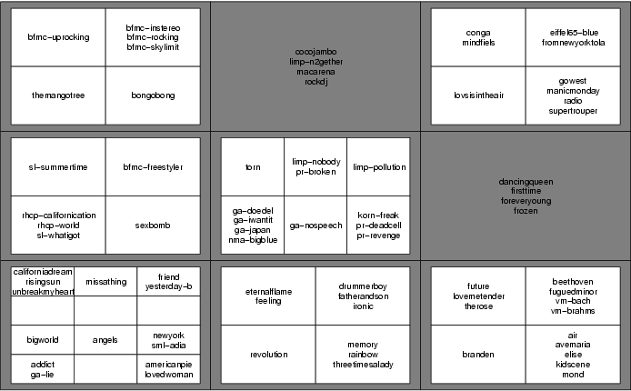The full title and artist to each identifier can be found here. On the first level the music collection has been divided into 9 categories. In this example, the bottom right represents mainly Classic music while the upper left mainly represents a mixture of Hip Hop, Electro, and House by Bomfunk MCs (bfmc). The upper-right, center-right, and upper-center represent mainly disco music such as Rock DJ by Robbie Williams (rockdj), Blue by Eiffel 65 (eiffel65-blue), or Frozen by Madonna (frozen). Some of these 9 first-level categories are further refined on the second level. For example, the lower right is divided into 4 further sub-categories. Of these 4 categories the lower-right represents slow and peaceful music, mainly piano pieces such as Für Elise (elise) and Mondscheinsonate (mond) by Beethoven, or Fremde Länder und Menschen by Schumann (kidscene). The upper-right represents, for example, pieces by Vanessa May (vm), which are modern interpretations of classical pieces. In the upper-left pieces with an music with an orchestra are located such as the as the end credits of the film Back to the Future III (future) and the slow love song The Rose by Bette Midler. Some interesting insights into the music collection which the GHSOM reveals are, for example, that the song Freestyler by Bomfunk MCs (center-left) is quiet different then the other songs by the same group. Freestyler was the groups biggest hit so far and unlike their other songs has been appreciate by a broad audience. Generally the pieces of one group have similar sound characteristics and thus are located within the same categories. This applies, for example, to the songs of Guano Apes (ga) and Papa Roach (pr), which are located in the center of the 9 first-level categories together with other aggressive rock songs. However, there is another exception, for example, Living in a Lie by Guano Apes (ga-lie) is located in the lower-left. Listening to this piece reveals that it is much slower than the other pieces of the group, and that this song which is about the end of a relationship matches very well to, for example, Addict by K's Choice which is about addiction to drugs. Back

		ghsom_demo5 Another application in the music domain is to analyse musical performances. See www.oefai.at/music for details. This demonstration illustrates how a 2-dimensional time series data can be clustered and visualized with the GHSOM. The time series are segmented to equal length. And each segment is represented by a vector of length 2*t where t denotes the number of time intervals. The first part of the vector (the first t elements) represent the x-value of the time series (in case of the music data this corresponds to the loudness [sone]) and the second part of the vector (the last t elements) represent the y-values (in this case tempo [bpm]) at each time interval t. load worms % load sData with musical performance data ghMap = ghsom_train(sData,'breadth',0.7,'depth',0.05,'tracking',2,'depth_dataitems',10) figure ghVisu = ghsom_visualize_grid(ghMap,'layer',1); ghsom_visualize_2dts(ghMap,ghVisu,sData,1); figure ghVisu = ghsom_visualize_grid(ghMap,'layer'); ghsom_visualize_2dts(ghMap,ghVisu,sData); The top layer GHSOM (2x2): 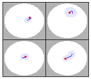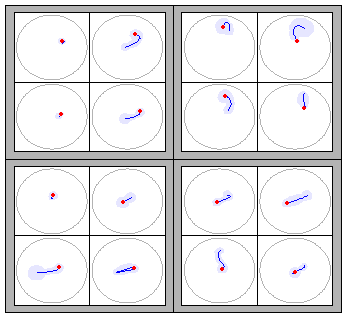The second layers (each 2x2): Back